
In this post we’ll use census data to cluster Australian federal electorates according to their demographic similarity. This is a good exercise for me to use some basic clustering algorithms, and it’s a component I’d like to use in my final model.
Remember that the important quantity in Australian parliamentary elections is the swing in each seat. If we can estimate the swing in each seat, we can assign seats using the Mackerras pendulum and get an election result.
Suppose we have come up with a nation-wide (or state-wide, or nation-wide but broken down by state) measure of swing. In a basic model, there may be an adjustment on a seat-by-seat basis based on a number of factors. Clustering seats together aims to eliminate this guesswork (such as assigning seats a classification like “rural” or “urban”). We will make small swing adjustments based on which clusters our seats belong to, calibrated by their mean collective swing as cluster at previous contests. As we mentioned in a previous post, this is all made much more complicated by redistributions.
Here I just want to choose the demographic variables we want to feed into the clustering algorithm, and come up with a sensible number of clusters.
Below is a list of the census demographic variables which for the 2006 census are most highly correlated with two-party preferred Labor vote at the 2007 Federal election (or equivalently with two-party preferred Coalition vote, since COA = 100 – ALP).
- Percentage of labour force in electorate aged 45 and above
- Migrant index (the migrant index is an average of four statistics which are presumably highly interdependent and which all have very similar correlation coefficients: percentage overseas born, percentage non-English speaking born, percentage speaking English badly or not at all, percentage speaking language other than English at home)
- Percentage of electorate employed in agriculture
- Percentage of electorate who are unemployed
- Median age in electorate
- Total dependency ratio
- Percentage of electorate aged between 15 and 24
- Percentage of electorate who are Catholic
- Logarithm of population density of electorate (The logarithm gives a more intuitive statistic given the highly skewed nature of Australian electorates and the rural/urban divide)
I thought the most interesting thing on this list was the first statistic, which had the highest correlation coefficient of -0.7267, and is plotted below:
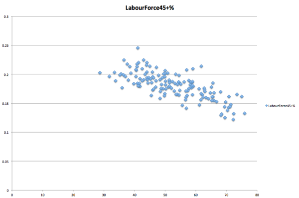
Personally, if I had to guess, I would have thought these two variables were positively correlated – persons over 45 in the labour force would seem to be prime candidates for old-school union movement Labor voters to me. But as you can see, the higher the proportion of the electorate in this category, the lower the Labor vote. And this relationship explains nearly 3/4 of the variance in 2PP Labor vote. There’s probably some confounding going on to explain this.
There is an obvious issue here that I’m only using data from 2006, which is nearly 10 years ago. I’m in the process of obtaining the 2011 census data by electoral district to see how these variables look at the 2013 election, but the ABS doesn’t make it as easy as it could. For the moment let’s just use these as a proof-of-concept.
So now we want to cluster seats according to these nine variables. This should provide a more sophisticated framework for swing and trend adjustment than I’ve seen in other models, which might take into account the rural/urban divide (which is accounted for mainly in variables 2, 3 and 5 above). They also usually take into account “sophomore surges” for members on their first reelection (variable 10 above); this is something I’ll talk about in another post.
I just want to use simple k-means clustering, and I’m going to use R. The main difficulty with k-means clustering is to choose the right value of k, the number of clusters. This requires a bit of trial-and-error to get right and needs to be calibrated against my own knowledge of Australian electorates.
The file I have here, called 2006_census_data_by_division.csv, is available in the GitHub repository. It took me a while to make, and contains columns for a bunch of interesting demographic variables, with rows labelled by the Commonwealth Electoral Divisions used in the 2007 election. I’m still in the process of making this work for the 2011 census data (which is harder to get at).
census <- read.csv('2006_census_data_by_division.csv')
pop <- as.numeric(as.character(census$Total_population[1:150]))
Need to do a whole bunch of coercion; notice that we convert to character before numeric otherwise we get the numeric value of the ASCII characters.
Var1 <- as.numeric(as.character(census$Labour_force_aged_45_years_and_over22[1:150]))/pop
Get the four variables that are part of our Migrant Index and average them up.
Mig1 <- as.numeric(as.character(census$Overseas[1:150]))
Mig2 <- as.numeric(as.character(census$NonEngBorn.[1:150]))
Mig3 <- as.numeric(as.character(census$Persons_who_speak_English_not_well_or_not_at_all[1:150]))/pop
Mig4 <- as.numeric(as.character(census$Persons_speaking_a_language_other_than_English_at_home[1:150]))/pop
Var2 <- (Mig1+Mig2+Mig3+Mig4)/4
Get the remaining variables.
Var3 <- as.numeric(as.character(census$Persons_employed_in_agriculture[1:150]))/pop
Var4 <- as.numeric(as.character(census$Unemployed_persons[1:150]))/pop
Var5 <- as.numeric(as.character(census$Median_age[1:150]))
Var6 <- as.numeric(as.character(census$Total_dependency_ratio3[1:150]))
Var7 <- as.numeric(as.character(census$Persons_aged_15_to_24_years[1:150]))/pop
Var8 <- as.numeric(as.character(census$Catholic.[1:150]))
Var9 <- log(as.numeric(as.character(census$Population_density1[1:150])))
divs <- census$division[1:150]
Put everything into a dataframe that allows us to cluster.
df = data.frame(divs, Var1, Var2, Var3, Var4, Var5, Var6, Var7, Var8, Var9)
If we start with two clusters, the algorithm seems smart enough to give us some sort of urban/rural divide.
two_clusters <- kmeans(df[,2:10],2)

two_clusters

K-means clustering with 2 clusters of sizes 94, 56
The differences between the means on Var3 and Var9 (workers in agriculture and population density, respectively) in the two clusters is illuminating:
> two_clusters$centers[,'Var3']
          1           2
0.002537473 0.033720529
> two_clusters$centers[,'Var9']
       1        2
6.789696 1.967118
as it gives a good picture of the urban/rural divide.
I think that a larger number of clusters will give a much more useful interpretation of what’s going on, and a more useful component to my eventual model. I want to use the largest number of clusters that gives a clustering so that I can still give some sort of qualitative description of each cluster (the way I’ve described the two clusters above as urban and rural). Let’s see if I can do this with six clusters.
In the spirit of including this as a piece in my Emma Chisit model, I translated this code to Python using scikit-learn (which also has a great out-of-the-box kmeans algorithm) and came up with the following groups:
- leafy outer suburban seats
- regional seats
- inner city seats
- poorer suburban seats
- wealthy suburban seats
- “Bigger than Peru” seats (Durack and Lingiari)
Trying with numbers larger than six gave me more groups than I could reasonably name, so these seem like good clusters to go with.